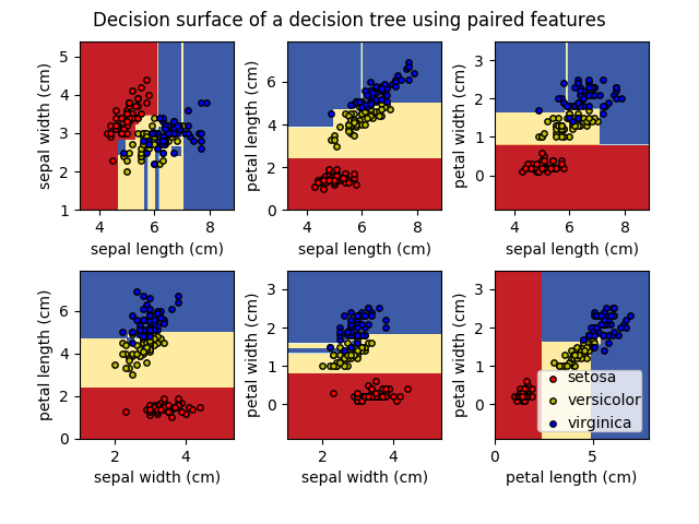
Plot the decision surface of a pruneable tree with pruning disabled

Plot the decision surface of a pruneabletree.prune.PruneableDecisionTreeClassifier trained on pairs of features of the iris dataset.

For each pair of iris features, the decision tree learns decision boundaries made of combinations of simple thresholding rules inferred from the training samples.

In this example, the tree is not pruned so it behaves the same as a regular DecisionTreeClassifier.

print(__doc__)

import matplotlib.pyplot as plt
import numpy as np
from sklearn.datasets import load_iris

from pruneabletree import PruneableDecisionTreeClassifier

# Parameters
n_classes = 3
plot_colors = "ryb"
plot_step = 0.02

def plot_surface(iris, prune_method):
    for pairidx, pair in enumerate([[0, 1], [0, 2], [0, 3],
                                    [1, 2], [1, 3], [2, 3]]):
        # We only take the two corresponding features
        X = iris.data[:, pair]
        y = iris.target

        # Train
        clf = PruneableDecisionTreeClassifier(prune=prune_method).fit(X, y)

        # Plot the decision boundary
        plt.subplot(2, 3, pairidx + 1)

        x_min, x_max = X[:, 0].min() - 1, X[:, 0].max() + 1
        y_min, y_max = X[:, 1].min() - 1, X[:, 1].max() + 1
        xx, yy = np.meshgrid(np.arange(x_min, x_max, plot_step),
                            np.arange(y_min, y_max, plot_step))
        plt.tight_layout(h_pad=0.5, w_pad=0.5, pad=2.5)

        Z = clf.predict(np.c_[xx.ravel(), yy.ravel()])
        Z = Z.reshape(xx.shape)
        plt.contourf(xx, yy, Z, cmap=plt.cm.RdYlBu)

        plt.xlabel(iris.feature_names[pair[0]])
        plt.ylabel(iris.feature_names[pair[1]])

        # Plot the training points
        for i, color in zip(range(n_classes), plot_colors):
            idx = np.where(y == i)
            plt.scatter(X[idx, 0], X[idx, 1], c=color, label=iris.target_names[i],
                        cmap=plt.cm.RdYlBu, edgecolor='black', s=15)

    plt.suptitle("Decision surface of a decision tree using paired features")
    plt.legend(loc='lower right', borderpad=0, handletextpad=0)
    plt.axis("tight")
    plt.show()

# Load data
iris = load_iris()

# Create plots
plot_surface(iris, prune_method=None)

Total running time of the script: ( 0 minutes 1.738 seconds)